Guides
Getting started
On this page · 9 sections
What you need
- Node.js 18 or later on the station PC (for the agent) and a current browser (Chrome, Edge, Firefox or Safari) anywhere on the network.
- The Scada Studio folder: studio/ with the designer, the runtime, the samples and the agent, next to the smart-industrial package it renders with.
Nothing is installed globally and nothing is compiled. The designer is a set of static files; the agent is one Node.js program without dependencies.
1. Start the agent
cd studio/agent
node agent.js
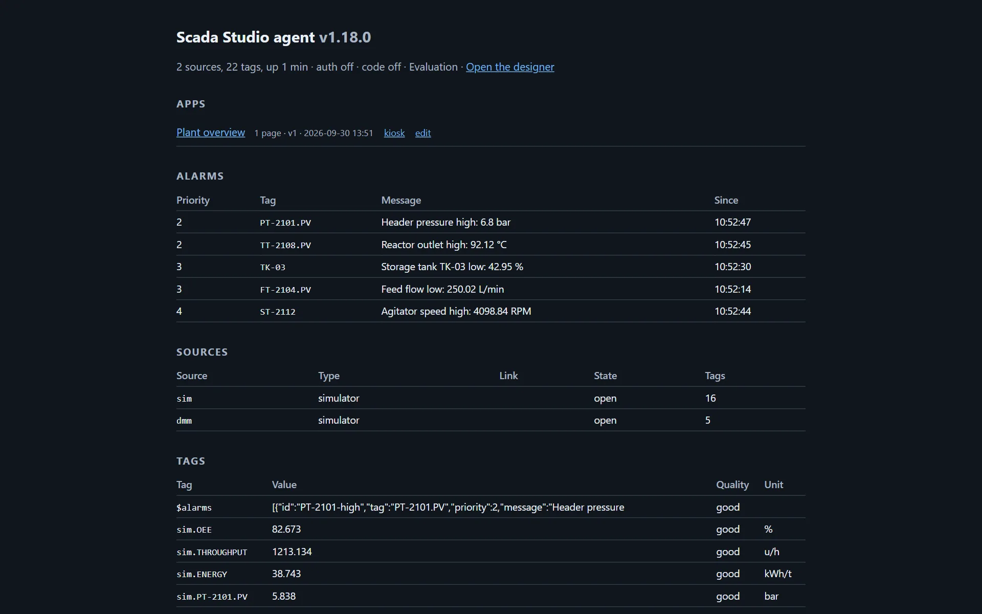
The agent starts with the configuration next to it, agent.config.json: two simulators - a process area of sixteen tags and a five-tag bench meter - so there is something to look at before a PLC is connected. It prints its address, http://localhost:8800/, where its home page lists sources, tags and apps. Open the designer there, or open studio/index.html from any web server.
Without any hardware
Nothing on this page needs an instrument. Two ways to have data:
- A simulated source in the designer (+ Source → simulator): tags with a shape, a range and a period. Good enough to build and demonstrate a whole screen.
- The bench instruments, which speak the real protocols on your own machine:
node studio/bench/instruments.js
That starts a Modbus TCP PLC (port 1502), a SCPI power supply (5025) and an HTTP gateway (8081), all measuring one small simulated plant: a temperature that follows its setpoint with lag, a flow that follows the pump, a motor that draws current. It prints the source definitions to paste into the station's configuration (sources); the designer then reads the instruments through the station, as an agent source. A setpoint written from a screen moves the temperature, because the instruments share the process - which is what makes it worth building a screen against. Nothing is written to disk and nothing leaves the machine.
This is the same path a real device takes: the station's Modbus, SCPI and HTTP drivers do not know the difference. Only the wire is missing.
2. Look at the sample
The designer opens on the plant overview - KPI tiles, three control loops, a trend, tank levels and five alarms evaluated live of one process area - and in front of it a gallery of the eight sample projects, each shown running: plant overview, alarm management, line operations, an andon board, a KPI wall, safety interlocks, a meter logger and the signal generator. Pick one to start from, keep the plant overview, or start blank; Project › New from a template… brings the gallery back.
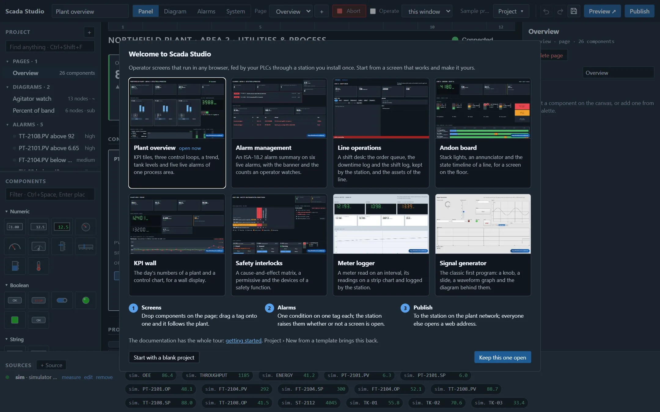
On the plant overview, drag a faceplate's setpoint (tick Operate): the request goes to the source and comes back confirmed, the way it would from a PLC. Open Alarms in the toolbar to see the five alarms that feed its banner and its Active alarms tile, evaluated as you watch. The samples are also the page templates (+ next to the page, start from).
The bar at the bottom lists the sources and their tags with live values. Drag a tag onto a component and its main property follows the tag; the Bindings tab in the inspector binds any property to any tag, with a unit conversion if the tag's unit differs from the display's.
3. Add your own data
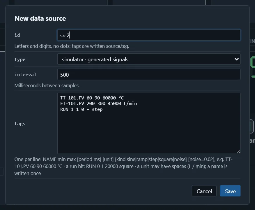
Press + Source. A simulator takes signals you describe (TT-101.PV 60 90 60000 °C, one per line). A websocket or sse source is a gateway that pushes samples; poll reads an HTTP endpoint on an interval. An agent source is a Scada Studio agent: enter its address (empty when the app will be served by the agent itself), press Fetch the agent's tags - on a station with users, sign in first (Publish or System › Live: the session is kept for the tab) - and the agent's PLCs and instruments are in the tag bar as agent.plc.TT-101.PV and so on.
To connect an instrument, pick it from the agent's templates in the same dialog (the instrument row: a Keysight 34461A, a Rigol DP800, a Keithley 2400…), give its address and press Add to the agent - the agent starts it and keeps it in its configuration. A PLC or anything else goes into the agent's agent.config.json, restart the agent; the source reference has every type, and the hardware page says what each has been run against.
4. Open the diagram
Open the signal generator from the gallery (Project › New from a template…) and press Diagram in the top bar. Its block diagram is there: a While loop every 200 ms reads the knob, the slide, the sample count and the switch through their terminals; a For loop computes the sine sample by sample and auto-indexes it into an array; the array goes to the graph's terminal and into Statistics for the RMS and the peak; a comparison lights the LED; the Stop button's terminal ends the loop. Press the run arrow: every node shows its last value under it, the wires pulse, and with the lightbulb on the values ride the wires. Add a node from the palette - the Front panel group has a terminal for each component of the page - wire it from a terminal on the right edge of one node to a terminal on the left edge of another (the colours must match: orange numbers, green booleans, pink text), set its fields in the inspector. A tag dragged from the bar onto the canvas becomes a Tag terminal.
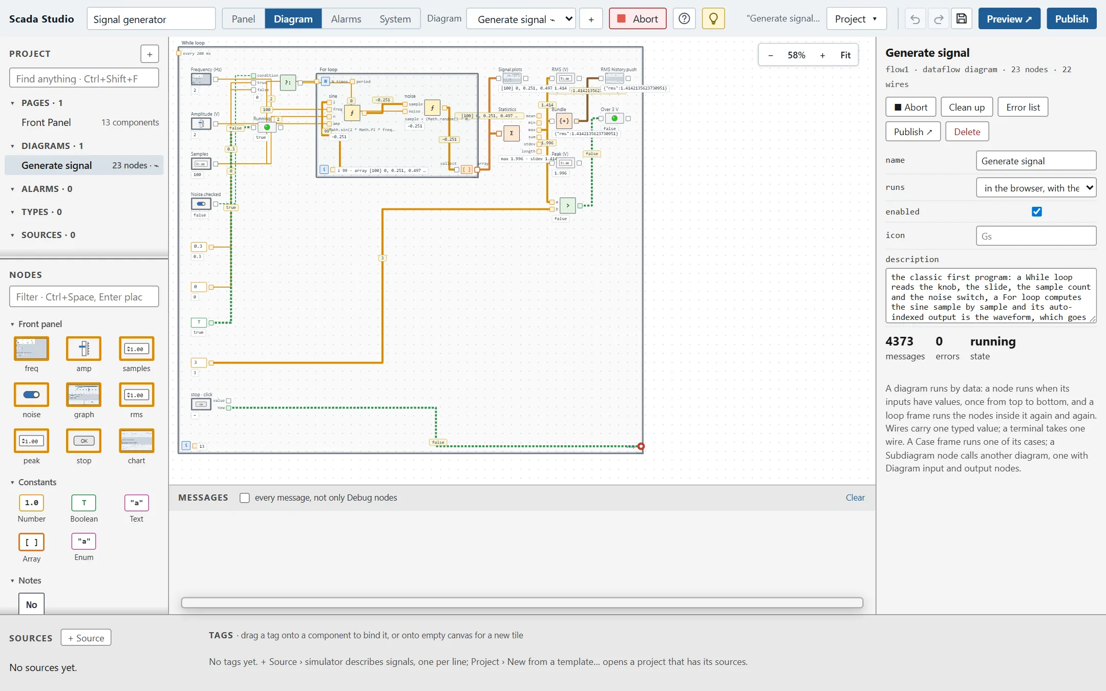
The diagrams guide has the rules, the frames and the look; the bench meter logger's second flow, Log every reading, is the other kind, a message flow that runs on the agent once the project is published, with or without a browser open, and logs to CSV. The plant overview sample has a Case frame choosing a stack light's state and a Subdiagram node calling a third diagram.
5. Publish
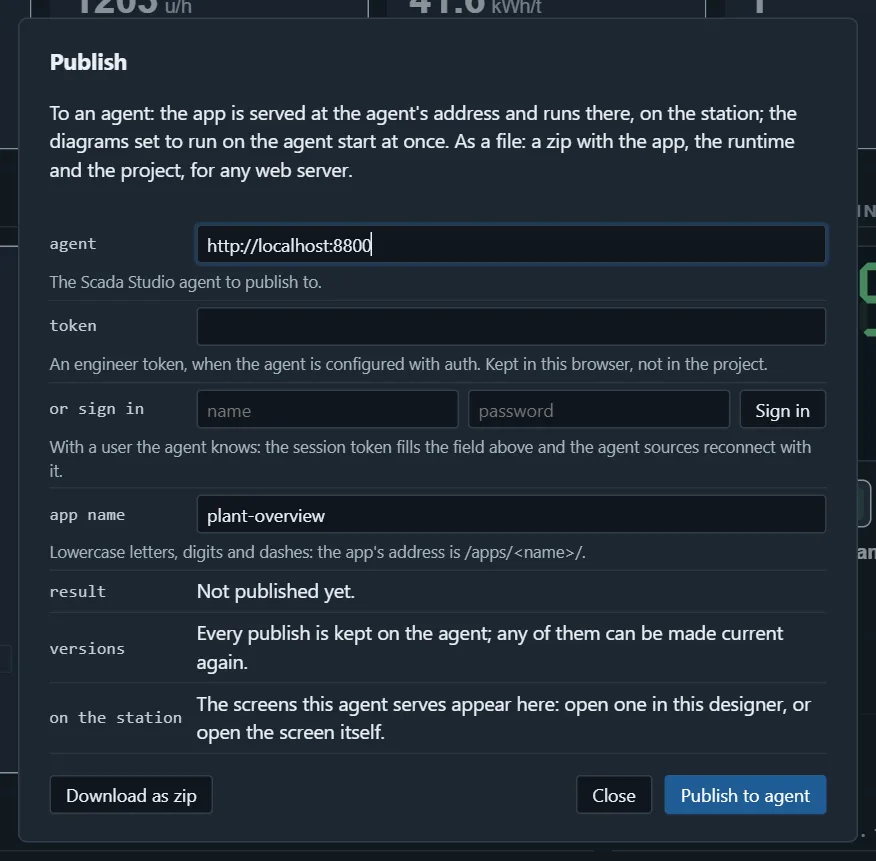
Preview opens the app in a new tab. Publish sends the project to the agent, which serves it at http://localhost:8800/apps/<name>/ and starts its agent-side diagrams; ?kiosk=1 on that address hides the page tabs for a screen on the wall. Download as zip gives a folder with the app, the runtime and the project for any web server.
6. Keep it
Save keeps the project in the browser; under Project, Export the project writes the project file, one JSON document that belongs in a repository, and Import a project… opens one. The project file is documented here.